Current Sense Resistor Essentials: Professional Insights for Accurate Circuit Design

In precision circuit design, few components carry as much weight as the humble current sense resistor. A slight miscalculation or subpar component choice can cascade into thermal drift, signal corruption, or outright failure. That’s exactly why understanding the nuances behind these resistors is non‑negotiable for engineers who push boundaries. At Milliohm, we’ve distilled decades of hands‑on expertise into practical guidelines that demystify selection, layout, and thermal management—insights you won’t find in generic datasheets. Whether you’re wrestling with high‑side sensing in noisy environments or squeezing micro‑ohm precision out of a budget‑constrained BOM, the right resistor strategy separates a stable design from a ticking time bomb.

Rethinking the Shunt: Beyond Resistance Value

For decades, the shunt resistor has been the go-to component for current sensing, valued for its simplicity and low cost. But focusing solely on the resistance value overlooks a web of interconnected performance factors. Thermal drift, parasitic inductance, and the physical layout of the sense connections can dramatically undermine measurement accuracy. A shunt is never just a resistor—it’s a precision element whose real-world behavior is shaped by temperature, frequency, and mechanical stress. Understanding these subtleties moves the design from a rough estimate to a reliable measurement.

Engineers often treat shunt selection as a trivial step: pick a value low enough to minimize power loss, yet high enough to generate a readable voltage. However, this trade-off is only the beginning. At high currents, the thermal mass and cooling of the shunt dictate its ability to maintain a stable resistance. Self-heating can push the resistor beyond its specified temperature range, causing permanent drift or even failure. Moreover, in alternating current or fast transient applications, the inductance of the shunt and its leads introduces an impedance component that distorts the sensed voltage, producing errors that no amount of calibration can correct if not mitigated at the design stage.

Stepping beyond the resistance value requires a systems-level perspective. The traces connecting the shunt to the amplifier form a Kelvin sensing layout, but their symmetry and proximity to noise sources determine the common-mode rejection. Even the choice of alloy—manganin, constantan, or metal foil—affects not just the temperature coefficient, but also the long-term stability and thermoelectric voltages at junctions. In precision instrumentation, the shunt must be considered a multi-physics component, where electrical, thermal, and mechanical design converge. Only by rethinking the shunt holistically can one achieve accuracy that truly matches the specifications on paper.

Precision Layout Tactics for Minimal Measurement Error

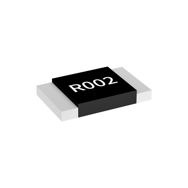
Every move of a probe or sensor introduces a risk of deviation. The trick lies in mapping out a path that avoids unnecessary travel while keeping each measurement point firmly within the instrument's sweet spot. It’s not about fancy algorithms—it's about understanding the physical dance between the tool and the part. Short, direct motions reduce the chance of drifting off target. Planning the sequence so the machine doesn’t have to double back or make sharp turns keeps the readings consistent. When every micron counts, a deliberate, almost cautious approach to layout pays off in repeatable accuracy.

Stability isn’t just a buzzword—it’s the foundation you build your measurement strategy on. Thermal changes, vibrations, even a wobbly table can twist a perfect setup into a mess of errors. Giving the equipment time to settle and keeping the environment steady matters as much as the layout itself. Think of it as letting the system catch its breath before you ask it to perform. Simple steps like positioning heavy fixtures closer to the base, using symmetrical patterns to balance load, and avoiding overhanging weights make the whole setup less jumpy. A layout that respects the physical limits of the gear naturally yields tighter tolerances.

Data points are only as good as the decisions that place them. Grouping critical measurements in a tight cluster minimizes the impact of any residual drift, while spreading out reference checks can catch errors before they cascade. There’s a rhythm to good layout: it alternates between taking a measurement and verifying against a known standard. This stitch‑in‑time approach means you’re not just collecting numbers—you’re building a web of cross‑checks that quietly corrects itself. Redundancy, placed thoughtfully, turns a fragile measurement chain into a resilient one without adding bulk to the process.

Thermal Drift Decoded: Managing Self-Heating Effects

At its core, thermal drift isn't some abstract gremlin—it's the silent performance killer born right inside your circuits. Whenever current pushes through a semiconductor, a fraction of that energy doesn't just disappear; it turns into heat, right at the junction. The hotter it gets, the more the electrical parameters start to wander. Think of it as a subtle, temperature-driven detuning of the device's own operating point. You might see your amplifier's quiescent current creeping upward, a sensor's zero-point shifting, or a precision timing circuit slowly losing its edge. The physics is straightforward: mobility drops, threshold voltages shift, leakage currents multiply, and suddenly the tight tolerances you designed for are out the window. It's especially brutal in high-density designs where power pulses concentrate in tiny areas for microsecond bursts—thermal time constants can't react fast enough, and localized hotspots form, dragging performance down in ways that are maddeningly non-linear.

Managing this isn't about slapping on a bigger heatsink and calling it a day. That's old-school thinking that ignores the dynamic nature of self-heating. What really works is a blend of smart layout, active compensation, and an intimate understanding of your thermal impedances. Start by spreading the power dissipation laterally on the die or board—interdigitated power devices, distributed resistive elements, anything that minimizes current crowding. Then think in the time domain: if you can't avoid a power surge, shape its envelope to give the material a chance to diffuse the heat before the next hit. On the circuit level, bake in feedback loops that sense the junction temperature rise (either directly with on-die diodes or indirectly by monitoring a drift-prone parameter) and nudge the bias or calibration accordingly. Some designers go further, using predictive algorithms that model the expected thermal trajectory based on recent loading history—essentially giving the system a memory of its own thermal past. It's a constant dance between power, time, and spatial layout, and when you get it right, thermal drift stops being a mystery and becomes just another variable you've tamed.

High-Frequency Nuances: Parasitics in Current Sensing

When you push a current-sensing circuit into the megahertz range, even the tiniest layout choices start to scream. A few millimeters of trace between the shunt resistor and amplifier isn’t just a wire—it’s an inductor that injects ringing and overshoot into your measurements. Those sharp switching edges that looked so clean on the schematic become jagged nightmares once parasitic inductance and capacitance start resonating. The result is a sense voltage that bears little resemblance to the actual current waveform, making accurate peak-current detection nearly impossible.

The shunt resistor itself hides unexpected gremlins. Above a few hundred kilohertz, its equivalent series inductance (ESL) dominates the impedance, turning a supposedly resistive element into a reactive one. Worse, the parasitic capacitance across the resistor terminals couples high-frequency noise directly into the amplifier input, creating a false differential signal. If the amplifier’s common-mode rejection isn’t stellar at those frequencies, the output becomes a mess of switching harmonics rather than a clean current replica.

Taming these effects demands more than just picking a “low-inductance” resistor. Kelvin sensing becomes mandatory to keep load-current-induced voltage drops out of the measurement loop, and the entire layout must be crafted with symmetrical, tightly-coupled traces to cancel magnetic fields. Burying guard traces between high-dV/dt nodes and the sense lines often saves a design from unexplained oscillation. Ultimately, accounting for parasitics at every copper pour and via transforms a temperamental high-frequency monitor into a trustworthy sensor.

Material Choices: Metal Alloy, Foil, or Thin Film?

Designing a flexible circuit starts with a fundamental question: what conductive material suits the application best? The decision between metal alloys, foils, and thin films is rarely clear-cut. It hinges on balancing cost, conductivity, mechanical fatigue, and the manufacturing process. For instance, a circuit that must endure repeated bending in a wearable device demands a completely different metallurgical profile than one buried inside a rigid smartphone component.

Rolled metal foils, often made from copper or aluminum, offer a practical middle ground. They bring excellent conductivity and can be etched into fine traces, yet they struggle with severe strain. In contrast, metal alloys like Constantan or Beryllium Copper are formulated for properties beyond basic conduction—think resistance stability or superior spring characteristics. These become vital when the circuit itself acts as a sensor or a connector, where slight variations in resistance or shape would compromise the entire function.

On the other hand, vacuum-deposited thin films represent a leap in precision. They allow for sub-micron thickness and the creation of intricate, multi-layer structures directly on flexible substrates. The catch? The process is expensive and often slower. It’s the go-to solution for high-density interconnects in medical catheters or OLED displays, where space is at an absolute premium and performance can’t be sacrificed. Ultimately, the material isn’t just about carrying current—it’s about shaping how, where, and for how long the circuit can live.

System-Level Calibration: Turning Measurements into Truth

Every measurement system carries inherent biases and uncertainties, but system-level calibration transforms raw data into reliable truths. Instead of focusing on individual sensor quirks, this approach views the entire measurement chain—from transducer to data logger—as an interconnected whole. By applying controlled reference standards across the system's operating range, we can map out and compensate for collective errors that single-component calibrations often miss. The result is a unified correction model that turns scattered measurements into coherent, trustworthy outputs.

Achieving this level of accuracy demands more than just periodic lab checks; it requires embedding calibration into the system's operational fabric. Modern techniques use real-time condition monitoring and adaptive algorithms to adjust for drift, temperature swings, and aging effects without stopping production. This continuous calibration loop ensures that what you read is always as close to the physical truth as possible, even in harsh industrial environments. By making calibration an active partner in the measurement process, we close the gap between the sensor's raw output and the actual state of the world it aims to capture.

FAQ

Conclusion

Accurate current sensing hinges on more than just picking a low-resistance shunt. Designers often fixate on the resistance value, but the physical layout can easily dominate measurement uncertainty. Kelvin connections, for instance, aren't a luxury—they separate current-carrying paths from voltage-sense lines, preventing PCB trace resistance from masquerading as shunt voltage. Even with perfect routing, thermal effects creep in. A resistor that self-heats under load doesn't just drift in value; it creates local thermal gradients that introduce Seebeck voltages at junctions, distorting the sensed signal. Mitigating this demands both derating and thoughtful placement, sometimes leveraging thermal vias or copper pours as heat spreaders. In essence, the shunt must be treated as a precision analog front-end, not a passive component.

Beyond DC performance, high-frequency behavior often blindsides designers. Shunt resistors exhibit parasitic inductance that turns a clean current waveform into a jumble of voltage spikes in switching converters. Selecting a low-inductance geometry—like a wide, short chip or a four-terminal design—curbs this, but understanding the current path's magnetic loop area is equally critical. Material choice then becomes pivotal: metal alloy elements handle pulse power with minimal drift, while foil technologies shine in ultra-low temperature coefficient applications, and thin film suits compact, high-precision circuits. Ultimately, no component is ideal. System-level calibration compensates for residual errors by mapping the entire signal chain, from shunt to ADC, against a known reference. This turns a good design into a trustworthy measurement, shifting the emphasis from component specs to end-to-end verification.